Distance Transform
The example in this section is present in the source under
mahotas/demos/distance.py.
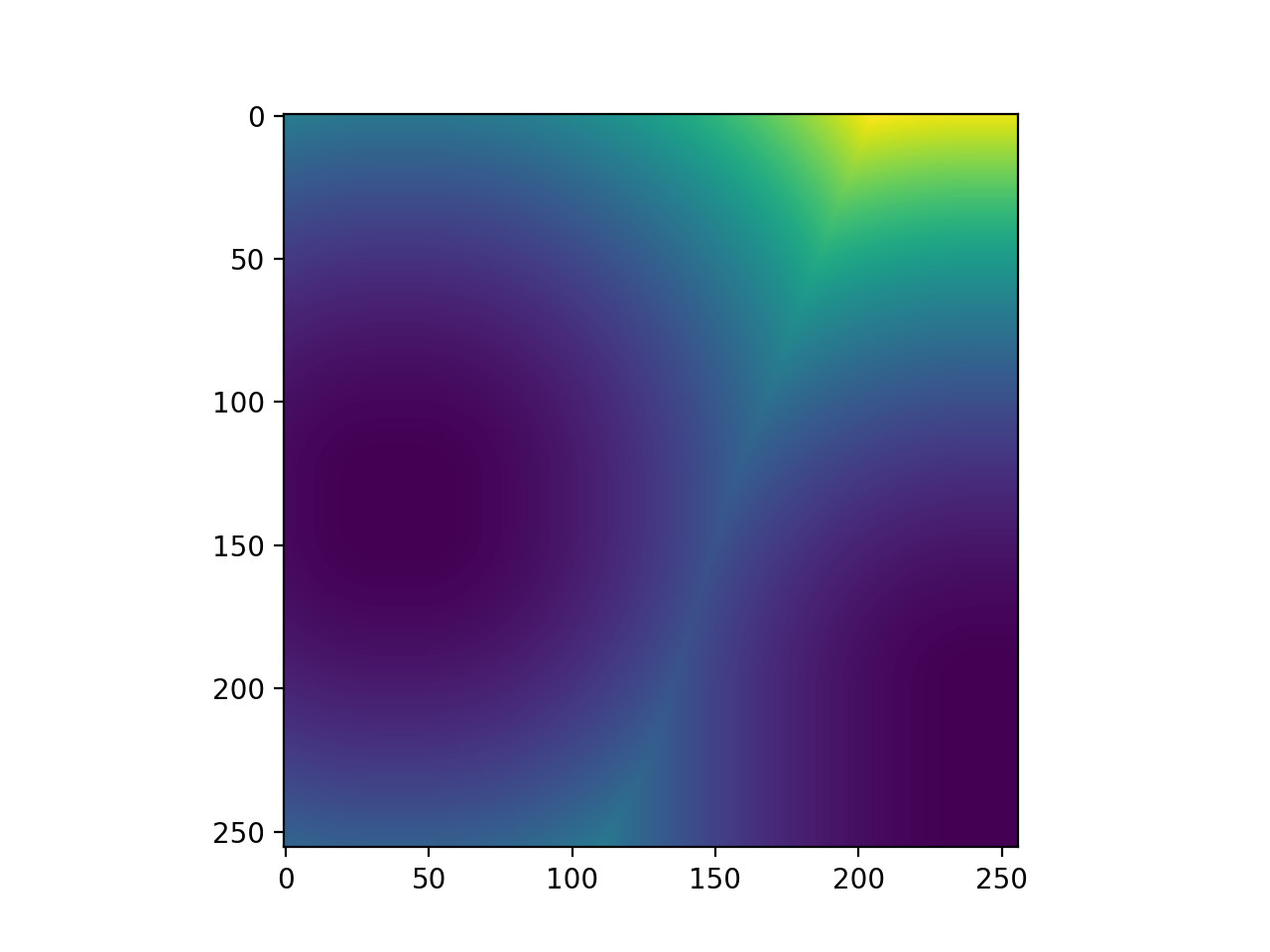
We start with an image, a black&white image that is mostly black except for two white spots:
import numpy as np
import mahotas

f = np.ones((256,256), bool)
f[200:,240:] = False
f[128:144,32:48] = False
from pylab import imshow, gray, show
import numpy as np

f = np.ones((256,256), bool)
f[200:,240:] = False
f[128:144,32:48] = False

gray()
imshow(f)
show()
(Source code, png, hires.png, pdf)

There is a simple distance() function which computes the distance map:
import mahotas
dmap = mahotas.distance(f)
Now dmap[y,x] contains the squared euclidean distance of the pixel (y,x)
to the nearest black pixel in f. If f[y,x] == True, then dmap[y,x] ==
0.
from __future__ import print_function

import pylab as p
import numpy as np
import mahotas

f = np.ones((256,256), bool)
f[200:,240:] = False
f[128:144,32:48] = False
# f is basically True with the exception of two islands: one in the lower-right
# corner, another, middle-left

dmap = mahotas.distance(f)
p.imshow(dmap)
p.show()
(Source code, png, hires.png, pdf)

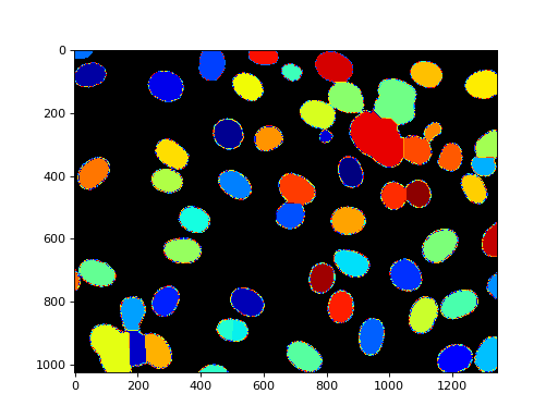
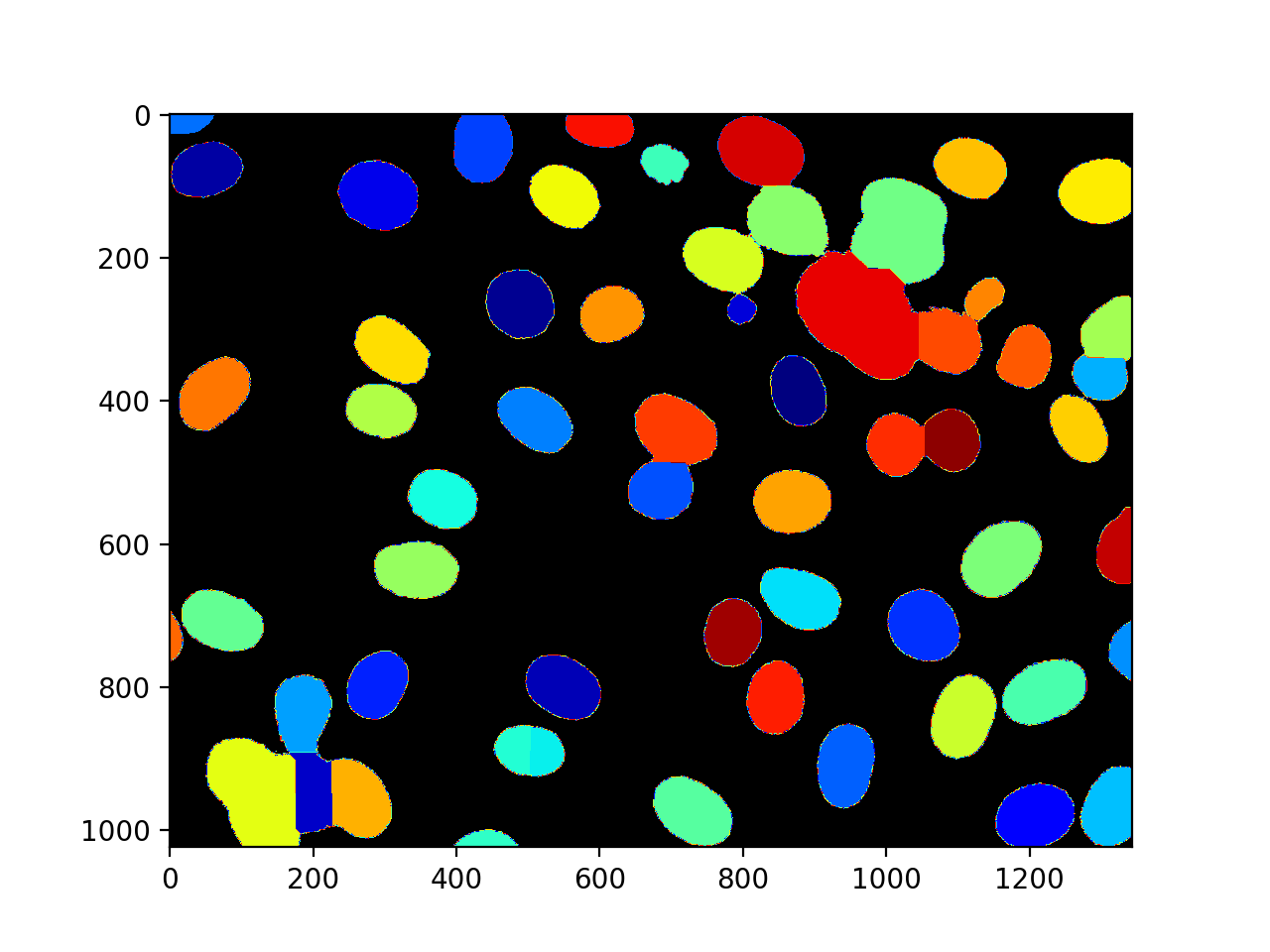
Distance Transform and Watershed
The distance transform is often combined with the watershed for segmentation.
Here is an example (which is available with the source in the
mahotas/demos/ directory as nuclear_distance_watershed.py).
import mahotas as mh
from os import path
import numpy as np
from matplotlib import pyplot as plt

nuclear = mh.demos.load('nuclear')
nuclear = nuclear[:,:,0]
nuclear = mh.gaussian_filter(nuclear, 1.)
threshed  = (nuclear > nuclear.mean())
distances = mh.stretch(mh.distance(threshed))
Bc = np.ones((9,9))

maxima = mh.morph.regmax(distances, Bc=Bc)
spots,n_spots = mh.label(maxima, Bc=Bc)
surface = (distances.max() - distances)
areas = mh.cwatershed(surface, spots)
areas *= threshed


import random
from matplotlib import colors
from matplotlib import cm
cols = [cm.jet(c) for c in range(0, 256, 4)]
random.shuffle(cols)
cols[0] = (0.,0.,0.,1.)
rmap = colors.ListedColormap(cols)
plt.imshow(areas, cmap=rmap)
plt.show()
(Source code, png, hires.png, pdf)

The code is not very complex. Start by loading the image and preprocessing it with a Gaussian blur:
import mahotas
import mahotas.demos

nuclear = mahotas.demos.nuclear_image()
nuclear = nuclear[:,:,0]
nuclear = mahotas.gaussian_filter(nuclear, 1.)
threshed  = (nuclear > nuclear.mean())
Now, we compute the distance transform:
distances = mahotas.stretch(mahotas.distance(threshed))
We find and label the regional maxima:
Bc = np.ones((9,9))
maxima = mahotas.morph.regmax(distances, Bc=Bc)
spots,n_spots = mahotas.label(maxima, Bc=Bc)
Finally, to obtain the image above, we invert the distance transform (because
of the way that cwatershed is defined) and compute the watershed:
surface = (distances.max() - distances)
areas = mahotas.cwatershed(surface, spots)
areas *= threshed
We used a random colormap with a black background for the final image. This is achieved by:
import random
from matplotlib import colors as c
colors = map(cm.jet,range(0, 256, 4))
random.shuffle(colors)
colors[0] = (0.,0.,0.,1.)
rmap = c.ListedColormap(colors)
imshow(areas, cmap=rmap)
show()
API Documentation
A package for computer vision in Python.
Main Features
- features
Compute global and local features (several submodules, include SURF and Haralick features)
- convolve
Convolution and wavelets
- morph
Morphological features. Most are available at the mahotas level, include erode(), dilate()…
- watershed
Seeded watershed implementation
- imread/imsave
read/write image
Documentation: https://mahotas.readthedocs.io/
Citation:
Coelho, Luis Pedro, 2013. Mahotas: Open source software for scriptable computer vision. Journal of Open Research Software, 1:e3, DOI: https://dx.doi.org/10.5334/jors.ac
- mahotas.distance(bw, metric='euclidean2')
Computes the distance transform of image bw:
dmap[i,j] = min_{i', j'} { (i-i')**2 + (j-j')**2 | !bw[i', j'] }That is, at each point, compute the distance to the background.
If there is no background, then a very high value will be returned in all pixels (this is a sort of infinity).
- Parameters:
- bwndarray
If boolean,
Falsewill denote the background andTruethe foreground. If not boolean, this will be interpreted asbw != 0(this way you can use labeled images without any problems).- metricstr, optional
one of ‘euclidean2’ (default) or ‘euclidean’
- Returns:
- dmapndarray
distance map
References
For 2-D images, the following algorithm is used:
Felzenszwalb P, Huttenlocher D. Distance transforms of sampled functions. Cornell Computing and Information. 2004.
Available at: https://citeseerx.ist.psu.edu/viewdoc/download?doi=10.1.1.88.1647&rep=rep1&type=pdf.
For n-D images (with n > 2), a slower hand-craft method is used.